
Choice of the best model
One of the most important phases of machine learning concerns the choice of the so-called “best model”.
Whether it is logistic regression, Random Forest, Bayesian methods, Support Vector Machine (SVM) or neural networks, there is no ideal model that can be defined as better than others, there is a “more adequate model” for the data and context in which we will go and operate.
Before addressing this very important topic, let’s make a brief introduction to Machine Learning.
Machine Learning (ML) is a branch within the wider world of Artificial Intelligence and aims to make machines automatically learn activities performed by us human beings.
The term Machine Learning was first coined in 1959 by Arthur Samuel and later taken up by Tom Mitchell who gave it a formal and current definition:
“It is said that a program learns from a certain experience E compared to a class of tasks T by obtaining a performance P, if its performance in carrying out the tasks T, measured by performance P, improves with experience E.”
There is a slight difference between the traditional algorithm and the machine learning algorithm.
In the first case, the programmer defines the parameters and data necessary for the resolution of the activity; in the second case, having to deal with problems for which there are no predefined strategies or a model is not known, the computer is made to learn by performing the activity and improving its execution.
For example, a personal computer program can solve the Tic-Tac-Toe game and be able to beat you because it has been programmed with a winning strategy to do so; but if he did not know the basic rules of the game, he would have to write an algorithm which, by playing, automatically learns these rules until he is able to win.
In the latter case, the computer does not just execute a “move” but rather tries to understand which could be the best: through the various examples it will get by playing it builds the rules that describe these examples and will be able to understand independently if the new case corresponds to the rule he has drawn and consequently will decide the move to be made.
Therefore, Machine Learning has the goal of creating models that allow you to build learning algorithms to solve a specific problem.
The learning model indicates the purpose of the analysis, that is, how you want the algorithm to learn.
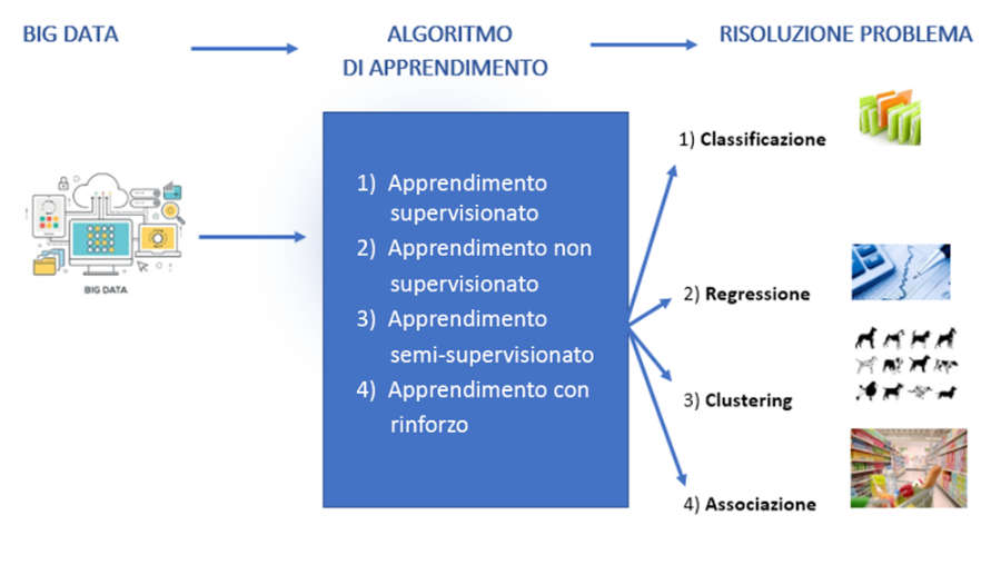
There are various learning models:
1) Supervised Learning
In this first case, the process of an algorithm learning from the training dataset can be thought of as a teacher supervising the learning process. Learning stops when the algorithm reaches an acceptable level of performance.
Supervised learning occurs when you have input data (X) and output data (Y) and an algorithm is used that learns the function that generates the output from the input.
The goal is to approximate the function so that when you have a new input data (X) the algorithm can predict the generated output value (Y) for that data.
Supervised learning problems can be divided into:
1) Classification: is the process in which a machine is able to recognize and categorize dimensional objects from a data set.
2) Regression: represents the fact that a machine can predict the value of what it is analyzing based on current data. In other words, it studies the relationship between two or more variables, one independent of the other.
For example, given the size of a house, predict its price, or look for the relationship between car races and the number of accidents a driver has.
3) Unsupervised Learning
Unsupervised learning is when you have an input variable (X), represented by data, and no corresponding output variable.
It aims to find relationships or patterns between the various data that are analyzed without using a categorization as seen for Supervised Learning algorithms.
Learning is called “unsupervised” because there are no correct answers and there is no teacher.
The algorithms are left to themselves to discover and present the interesting data structure.
Unsupervised learning problems can be divided into:
3.1) Grouping: also called “clustering”, it is used when it is necessary to group data with similar characteristics.
In this case, the algorithm learns, if and when, it identifies a relationship between the data.
The program does not use previously categorized data but extracts a rule that groups the cases presented according to characteristics it derives from the data itself.
The program does not specify what the data represents and for this reason it is more complex to determine the reliability of the result.
3.2) Association: it is a problem in which you want to discover rules that describe large portions of the available data such as, for example, people who buy a product A also tend to buy a product B.
It aims to find frequent patterns, associations, correlations or random structures between a set of items or objects in a relational database.
Given a set of transactions, it tries to discover rules that predict the event of an item based on the events of other items in the transaction. It is closely related to Data Mining.
4) Reinforcement Learning
Machine learning technique that represents the computerized version of human learning by trial and error.
The algorithm lends itself to learning and adapting to environmental changes through an evaluation system, which establishes a reward if the action performed is correct, or a penalty in the opposite case.
The goal is to maximize the reward received, without announcing the path to take.
After this introduction to Machine Learning and the various training models, let’s face the issue of choosing the right model based on data and knowledge.
Over time, each training model has evolved on various more or less complex and sophisticated algorithms.
The production of a good model is critically dependent on the selection and optimization of features, as well as the selection of the model itself.
The process of identifying the best model is a complex and iterative process.
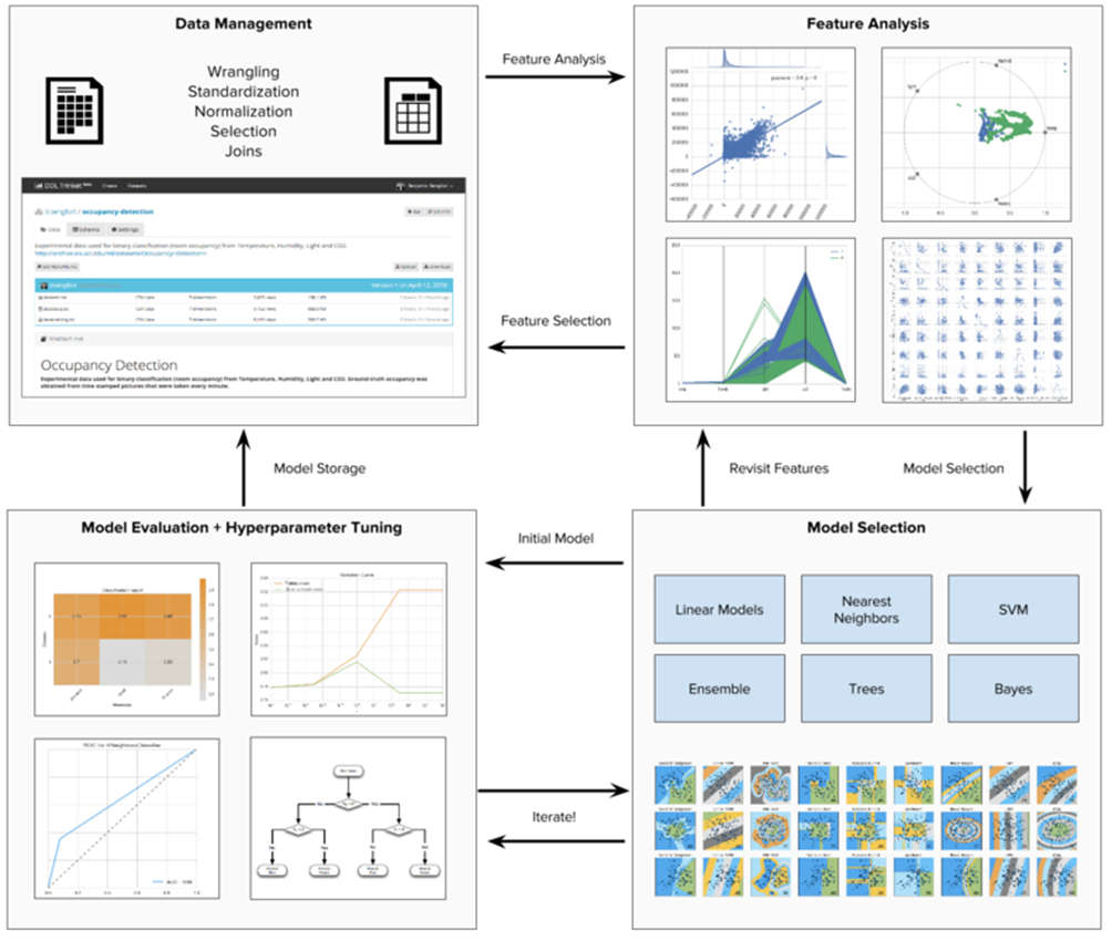
As shown in the diagram, we start with analyzing the characteristics using histograms, scatter plots, and other visual tools. This important phase is called EDA (Exploratory Data Analysis)
Then the analysis of the data characteristics is carried out, where normalizations, resizing and extraction of attributes are performed.
After this phase, which allows us to analyze the data and understand the context, we identify the category of machine learning models that best suits the objectives and the problematic space, often experimenting with the prediction of adaptation on multiple models.
This step is iterated between evaluation and tuning using a combination of numerical and visual tools such as ROC curves, residual plots, heat maps and validation curves.
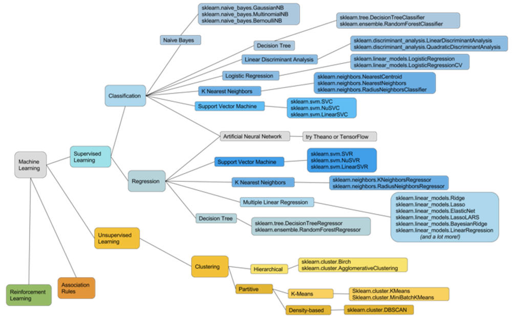
One of the methods we use during this phase of choosing the model is described by the Scikit-Learn library through the use of the following diagram.

This diagram is useful for a first step, as it models a simplified decision-making process for selecting the most suitable machine learning algorithm for your dataset.
The Scikit-Learn flowchart is useful because it gives us a map, but it doesn’t offer much in the way of transparency about how the various models work.
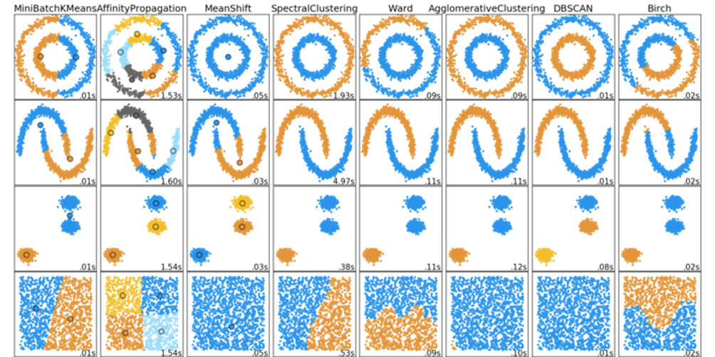
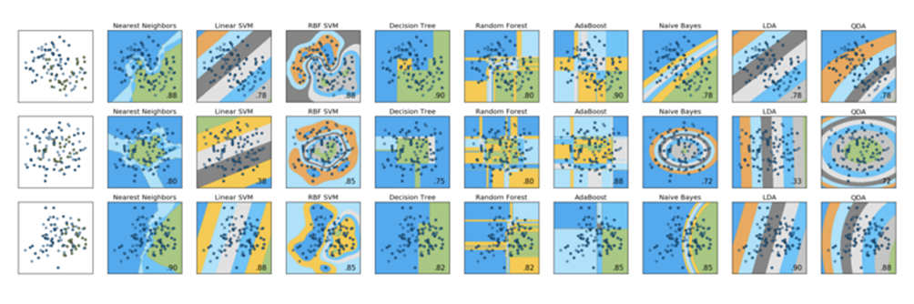
For this kind of insight, there are two images that have become somewhat canonical in the Scikit-Learn community: the classifier comparison and the clustering comparison graphs.
Since unsupervised learning runs without the benefit of having the data labeled, the “clustering comparison” chart is a useful way to compare different clustering algorithms across different data sets:
Similarly, the ranking comparison chart below is a useful visual comparison of the performance of nine different classifiers across three different data sets:
Typically these images are used only to demonstrate substantial differences in the performance of various models between different data sets.
But what do you do when you’ve run out of all those options? There are a lot more templates available in Scikit-Learn, and the previously seen flowchart is barely the surface. You can use a comprehensive approach to essentially test the entire Scikit-Learn model catalog in order to find the one that works best on your dataset.
But if our goal is to be more knowledgeable “Machine Learning professionals”, then we care not only about how our models work, but why they are, or aren’t, working.
For our purposes, experimentation, within the model modules, and the “hyperparameters”, is probably the place to get the best model choice. One tool that is used for model exploration is Dr. Saed Sayad’s interactive data mining map.
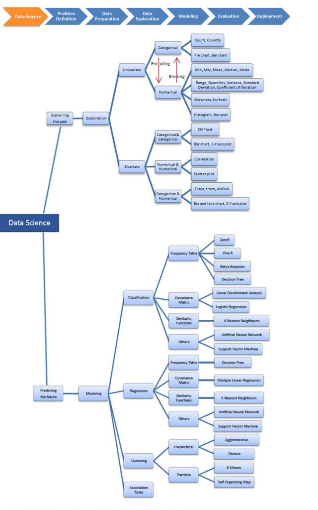
https://www.saedsayad.com/data_mining_map.htm
Much more comprehensive than the Scikit-Learn flowchart as it integrates other models and also, in addition to predictive methods, includes a separate section on statistical methods, the exploration (EDA) and data normalization part.
Below is an iteration on a graph that we created in Humanativa R&D Department, and which aims to present the same broad coverage of Sayad’s predictive methods (representing some of them, such as reinforcement learning, not represented in the original), while integrating the Scikit-Learn diagram.
Color and hierarchy define the model shapes and model families:
Although this map is not complete, the goal is for it to become a tool that, based on our experience, will allow us to select the models to be tested faster on the basis of the available data.