In the previous article we described in general the functioning of neural networks, in this second publication we will analyze in detail the “Convolutional Neural Network” (CNN), a type of feed-forward neural networks.
Convolutional neural networks are born from studies conducted on animal prefrontal cortices and have been used in image recognition processes since 1980.
In the CCNs, filters are applied that recognize particular correlations or patterns within the image itself, in order to generate optimal features to be supplied as input to a neural network (usually fully-connected).
From the mathematical point of view, the convolution operation consists in “multiplying” two matrices suitably translated to calculate the result, one of which represents the image being analyzed and the other the filter that is applied.
With convolution operations it is possible, in fact, to apply specific filters to extract a set of information. For example, in image recognition you could extract the left edges with the first filter, the right ones with the second, the corners with the third etc. … until the optimum accuracy level is reached.
In the process of convolution, we have three fundamental elements:
- The input image: an array of pixels representative of the image. For example, let 32×32 display a number, letter, or icon.
- The feature detector or Kernel: a matrix that acts as a filter through the convolution operation. For example, 3×3 or 7×7.
- The feature map: the matrix resulting from the convolution between the input image and the Kernel.
At the end of this process, you get the feature map, a smaller matrix than the input image.
For example, filtering a 32×32 image with a 7×7 kernel gives a resulting array of size 26×26.
In the convolution process, some information on the image is lost (the ones not contained in the chosen feature detector or kernel). However, that information will be contained in other future maps.
In fact, using multiple convolution filters you will get multiple feature maps, each of which will store distinctive features of our image, such as the right outline, edges, darker colors etc.

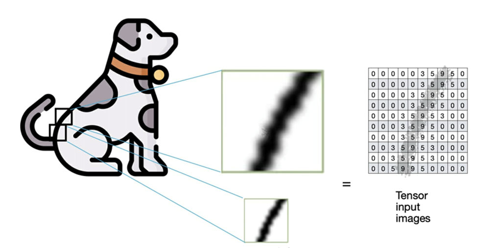
In the figure the image of the dog is encoded obtaining the input matrix.
In reality, a series of training images will be passed to the CNN algorithm as input, together with a matrix vector also called Tensor.
As mentioned, if several filters are applied to the input matrix representative of the image, with multiple convolution operations, a series of feature maps will be obtained.
The feature maps obtained are “sub-sampled” through a process called pooling.
Pooling is the technique that allows you to reduce complexity by considering only a part of the data.
This is a dimensional reduction process that simplifies the complexity of a CNN.
There are two pooling techniques: max pooling and average pooling. In practice, operations are carried out to calculate the maximum or average value on a subset of boxes of the input matrix. The goal of pooling is to minimize complexity, thus reducing overfitting.
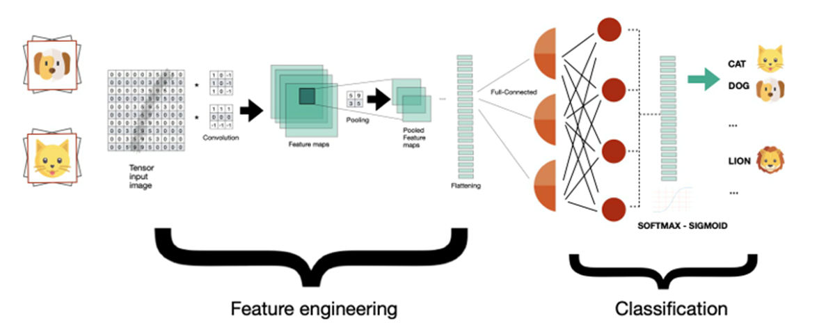
The convolution process and the subsampling process by pooling are both repeated, among other things by applying nonlinear activation functions to the various feature maps, namely the Rectified Linear Unit (RELU).
After N convolution processes – Pooling – RELU, you will need to transform the pooled feature maps into a one-dimensional vector, using the process called Flattening.
It will thus be possible to provide the resulting vector as input to a fully connected neural network, where each node will be connected with all the others: this is in practice the hidden level of our CNN that deals with the prediction and classification of the image.
At the end of the process, we will reach the output layer, where two types of activation functions will be applied to complete the image classification: the sigmoid function in case of binary classification, or its multi-dimensional variant called softmax, suitable in case of classification related to multiple categories.

Analyzing the previous figure, the CNN network is divided into two processes:
- The first contains the initial layers where features are prepared using convolution, pooling, and flattening processes. The goal is to extract image features that are presentable to the next process, the neural classification network.
- The second process consists of a traditional neural network, in our case completely connected to better classify the image based on the features received as input.
By clicking on the link below you can see an example of CNN with convolutional network in 2D: https://www.cs.cmu.edu/~aharley/vis/conv/flat.html
Humanativa Projects
One of Humanativa’s still ongoing projects in the CNN field is focused on the possibility of extracting information about faces, objects and locations from a video file (films / documentaries).
The result of this project will then be used to implement research image services to extract additional information from search engines.

