
Introduction
In this article, we report an excerpt from an experiment conducted in 2022 on passenger flow data at the Point Of Interest (POI) of a national transport location. In particular:
- we will display the results of Forecast models for a single POI, obtained through a Machine Learning framework conceived, designed and developed at Isiway.
- we will compare the results with a baseline based on real flows and the model in use at the transport location chosen for the experiment;
- we will illustrate a simulation of an MLOps service in order to demonstrate the effectiveness of a monitoring strategy accompanied by an on-line learning procedure based on an alert trigger on the performance of the model in production.
In this case, a forecast model is not simply a model that performs adequately with respect to a literature metric adopted as a reference for the evaluation of results but must be a model that solves a well-defined business problem: the optimization of personnel management at a POI as a function of passenger flows.
Materials and methods
The data made available for the chosen access point were used, showing, for the period from 2019 to 2021 and at five-minute intervals, the actual passenger flow at the access point and the estimate provided by the internal forecast model.
The forecast models presented here are developed through the Forecast Engine, a Machine Learning framework in the Python language, conceived, designed and developed at Isiway (Humanativa Group) for the automation of the process of importing, exploring data and generating models. The engine’s functionalities are in line with the AutoML processes made available by cloud providers.
The framework operates on the basis of the various libraries available in the literature, from those of classical statistics to more recent ones based on the paradigm of deep learning and recurrent neural networks and is continuously being expanded on the basis of recent developments proposed by the scientific community.
The following figure shows its functionalities.
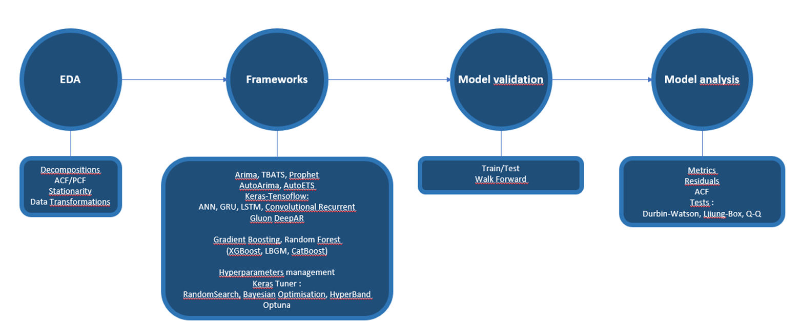
Figure 1. the Forecast Engine framework
The EDA module provides the following functionalities:
- Time Series decompositions (classical and STL)
- AutoCorrelation Function and Partial Correlation Function, for autocorrelation lag analysis used in classical statistical models of the ARIMA type
- Stationarity tests
- Transformations of the data based on the tests (e.g. BoxCox)
Available forecast models are:
- Arima, AutoArima
- TBATS
- ETS, AutoETS
- Prophet
- From TensorFlow: ANN, GRU, LSTM, CNN
- From GluonTS: GluonDeepAR
- Gradient Boosting and Random Forest (from the XGBoost, LightGBM and CatBoost libraries)
Hyper-parameterization procedures are based on:
- Keras Tuner (Random Search, Bayesian Optimization and HyperBand)
- Optuna
The developed models are analyzed through:
- Metrics (e.g. RMSE, R2)
- Analysis of residuals, with Durbin-Watson, Ljiung-Box and Q-Q tests
- AutoCorrelation Function.
The model development protocol is shown in the figure below.
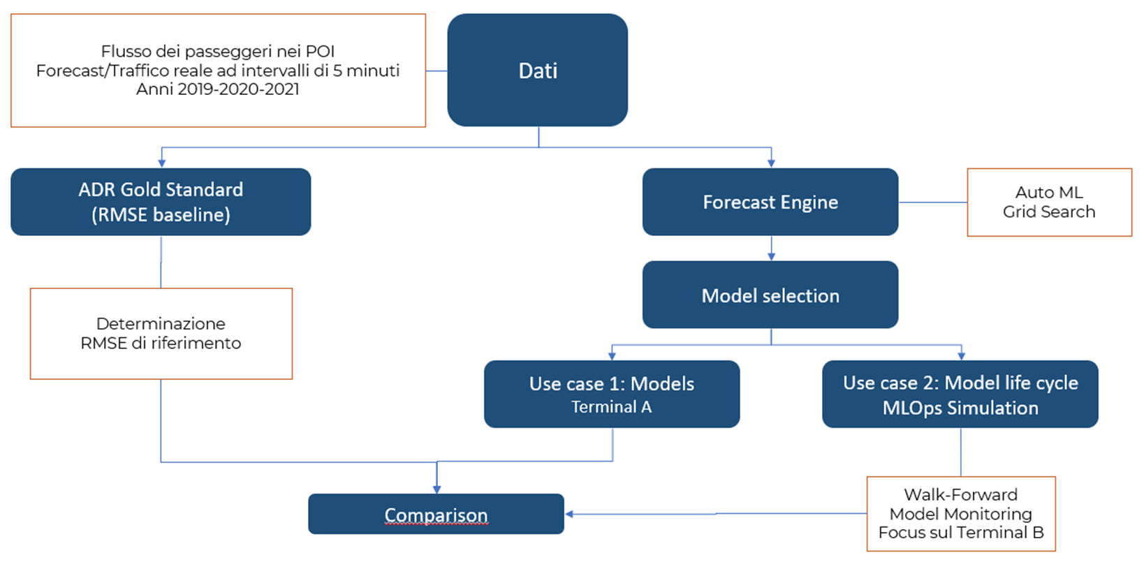
Figure 2. Analysis Protocol
The first stage of the protocol is the definition of a Gold Standard, a metric that can be used as a baseline for the proper evaluation of the model produced by the Forecast Engine. In the figure below, we show the metrics available for a forecast problem, and in particular the metric adopted, the RMSE.
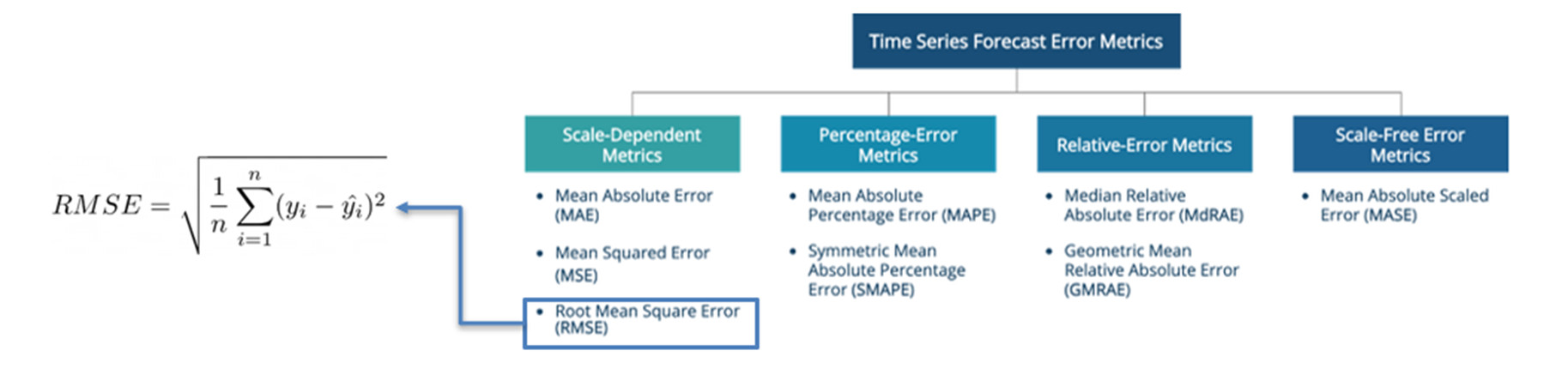
Figure 3. Forecast Metrics
The Root Mean Square Error (RMSE) has the following advantages:
- it is expressed in the same units as the data.
- it is easily calculated.
- it allows comparison among different models based on the criterion that the errors have a normal distribution.
As anticipated, we will report the results of what is referred to as Use Case 2 in Figure 2, since in this case we have simulated a Machine Learning Operations process (today commonly referred to as MLOps), articulated in the Monitoring and Continuous Delivery phases which makes it possible to automate the control of the model in production and the possible need to develop a new one in the event of performance degradation, generally due to data drift. This type of model management is now made available by all cloud providers.
In short, we have adopted the Rolling Origin Walk-Forward model validation protocol in the production phase, evaluating the model at each new data input and defining a performance degradation alert trigger based on a threshold set on the RMSE.
Validation of a forecast model using the Walk-Forward protocol is the gold standard for the study of time series and corresponds to the k-fold cross validation method in the context of supervised model development. At each step, the model produced from a training sample of fixed size is validated on a sample consisting of subsequent training data of fixed size. Both samples “run” over time according to a fixed interval. At each step, the quality of the model is verified and the final metric that defines the overall performance of the model is simply an average.
If the origin of the training sample is fixed, at each step in the process the sample will expand, as illustrated in the figure below.
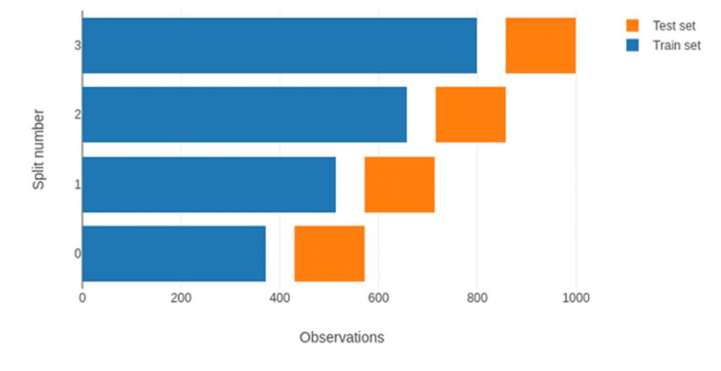
Figure 4. Walk-Forward validation protocol with expanding window
If the origin of the training sample is set as rolling origin at the beginning of the process, the training sample will have a fixed size and its time interval will be redefined at each step.
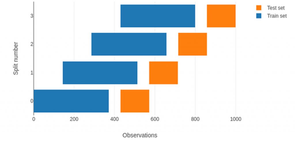
Figura 5. Walk-Forward validation protocol with rolling origin.
Experimentation
The analysis described here is structured in three phases:
- development of a model on the 2019 data (‘2019 model’);
- inference of the model on the 2020 and 2021 data to check its robustness;
- implementation of the MLOps simulation.
Model development
The time window defining the number of input features, derived from the reframing of the problem as supervised, is given by a lag number of 288 (number of detections in one day with 5-minute sampling).
Using the Forecast Engine, we defined a series of tests based on the algorithms shown in Table 1.
| N, | Model |
| 1 | Keras Sequential |
| 2 | Keras Sequential (Deep Learning) |
| 3 | Sequential with Tuner (Tuner Hyper-Parameters Optimisation) |
| 4 | Gated Recurrent Unit 1 (GRU) |
| 5 | Gated Recurrent Unit 2 (GRU) |
| 6 | Long Short Term Memory 1 (LSTM) |
| 7 | Convolutional Recurrent (CNN-GRU, Experimental) |
| 8 | Gradient Boosting XGBoost 1 |
| 9 | Gradient Boosting XGBoost 2 |
| 10 | Gradient Boosting XGBoost_RandomForest |
| 11 | Gradient Boosting CatBoost (Optuna Hyper-Parameters Optimisation) |
Of course, the process definition of models can be considerably extended. Here, we would like to emphasise not only the results obtained, but also the methodology of model development.
The best performing model is a Sequential neural network (Keras) with two hidden layers. The architecture is shown in the figure below.
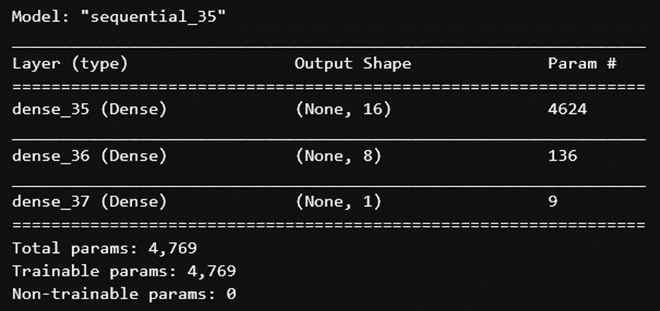
Figure 6. Sequential model architectures with best performance
The results are shown in the table below, in which the results on the training sample are also shown in order to check for overfitting or underfitting.
| RMSE | MAE | MSE | R2 | R2Adj | |
| Train | 17.272 | 10.442 | 298.33 | 0.924 | 0.924 |
| Validation | 8.615 | 5.503 | 74.214 | 0.854 | 0.853 |
The evaluation module of the results, provided by the Forecast Engine, provides the following three analyses:
- Residual Analysis. These must be uncorrelated (the presence of correlations indicates the presence of information that the model did not intercept) and must be i.i.d., have a normal distribution with zero mean and constant variance.
- Durbin-Watson test, whereby a value close to 2.0 indicates that there is evidence of autocorrelation.
- ACF (autocorrelation function). Values should be close to zero: 95% of the spikes should be in the range ±2/√T where T is the length of the time series
Figure 7 shows the analysis of the residuals. The Durbin-Watson test indicated a value of 1.81, whereby the residuals show no significant evidence of autocorrelation.
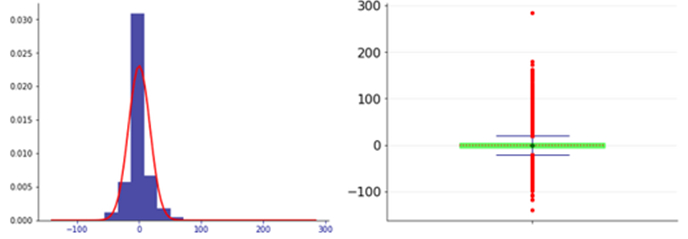
Figure 7. Distribution of residuals
Figure 8 shows the graph of the AutoCorrelation Function, which highlights the overall goodness of the model.
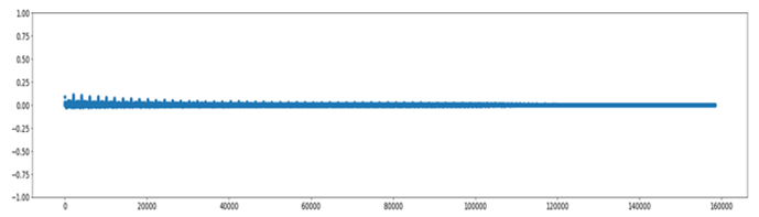
Figura 8 ACF.
Inference of the model on 2020 and 2021 data
Year 2020
The value of the RMSE is 7.32 and the Durbin-Watson test shows a value of 1.73.
The following figures show the residual analysis and the ACF respectively.
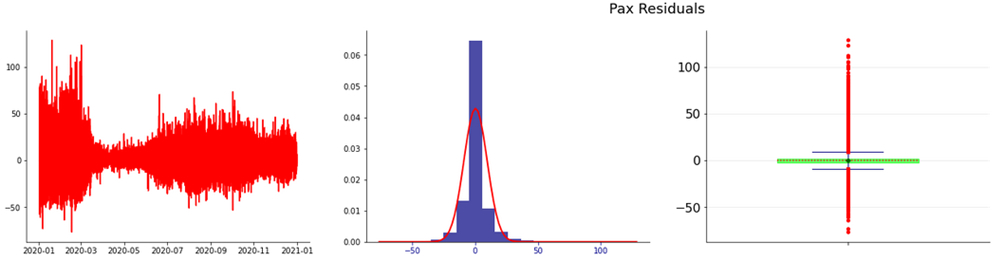
Figure 9. Residuals and Distribution of Residuals
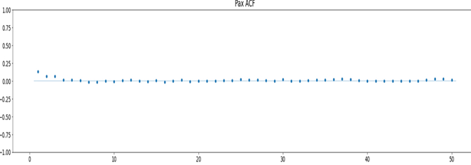
Figura 10 ACF
Year 2021
The RMSE value is 8.50 and the Durbin-Watson test shows a value of 1.81.
The following figures show the residual analysis and the ACF respectively.
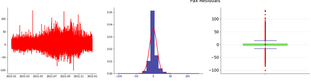
Figure 11. Residuals e Residuals Distribution
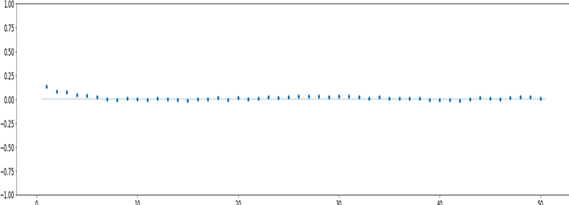
Figure 12. ACF
The table below shows the overall results, which show that the model based on 2019 data is still holding up well.
| Model | RMSE | Durbin-Watson |
| 2019 | 8.61 | 1.81 |
| 2020 | 7.32 | 1.73 |
| 2021 | 8.50 | 1.81 |
MLOps simulation
The protocol is based on the following steps:
- ‘Model 2019’ in production;
- Determination of a threshold related to the value of the RMSE above which the model is considered not to be performant;
- Inference on the data of the following 24 hours;
- Rolling origin: the time window of the training sample is shifted by 24 hours using the real data stream;
- Monitoring of the ‘2019 model’ without updates;
- Monitoring of the model with update trigger:
- If the RMSE of the model on the current data is below the threshold, the model is confirmed;
- If the RMSE of the model on the current data is above the threshold, a performance degradation event is triggered: in this case, a learning phase must be initiated in order to develop a new model whose performance must be below the threshold. Updating the model is mandatory in the event of a data drift, due to external events (such as pandemics or economic crises). This option allows the problem to be resolved promptly. Of course, it is a more onerous procedure, but it allows an adequate level of model performance to be maintained.
- If the on-line model update procedure does not produce the desired model, a new model production run through the Forecast Engine (off-line) is required with a data analysis to highlight the reasons for the degradation of the model in production.
Monitoring of the “2019 model” without updates
In this case, we want to check the robustness of the ‘2019 model’ on the data of the years 2020 and 2021 with a Walk-Forward validation procedure and a reference threshold set at 10.0, without performing a new learning phase.
The following figure shows the performance of the simulation.
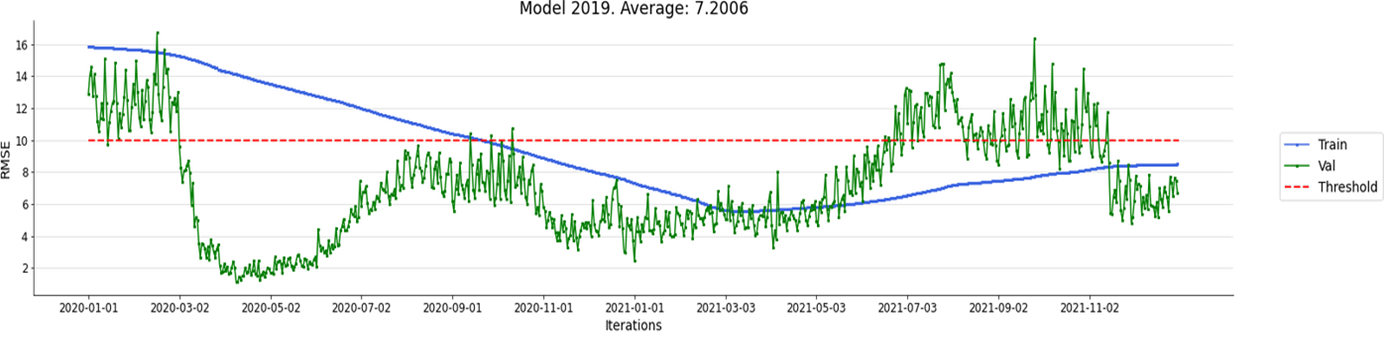
Figure 13. Validation of 2019 Model without updates
Performance is good: the average RMSE is 7.2. The 10.0 reference threshold adopted is very strict, but the choice was made to verify the improvement due to the Walk-Forward protocol. The threshold value was exceeded until 13 April 2020 on the training sample and on 167 times on the validation sample in 2021.
Monitoring of the ‘2019 model’ with online updates
Figure 11 shows the performance of the simulation with update triggers, in order to test the performance improvement hypothesis against the “2019 model” throughout the analysis interval from 2020 to 2021. The reference threshold (RMSE) set is 10.0.
As might be expected, the improvement over the ‘2019 model’ is clear, for both samples. The RMSE is still below the reference threshold and the overall average is 4.68 compared to 7.2 in the ‘2019 model’.
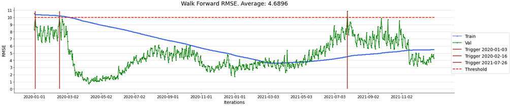
Figure 14. Validation of 2019 Model with updates
Performance degradation triggers were only triggered on three occasions, as shown in the table below.
| Data Trigger | RMSE pre-update | RMSE post-update |
| 2020-01-03 | 10.043 | 8.707 |
| 2020-02-16 | 10.16 | 9.22 |
| 2021-07-26 | 10.8 | 8.82 |
It is interesting to note the dynamics of the RMSE of the relevant triggers during the period in which the Covid-19 pandemic led to a reduction in traffic based on lockdown policies. The continuous learning strategy in production proposed here proves effective in ‘reacting’ to the variable dynamics that marked the year 2020 and the ‘post-pandemic’ phase of 2021.
Comparison with the original baseline
The table below shows the baseline of the RMSE metric calculated on the available data, for each year and for the entire period 2019-2021.
| Year | RMSE |
| 2019 | 27.11 |
| 2020 | 16.08 |
| 2021 | 19.5 |
| 2019-2021 | 21.74 |
The figure shows the comparison on a monthly basis between:
- the results of the protocol with the fixed, non-updatable ‘2019 model’;
- the results of the protocol with the “2019 model” with online Walk-Forward based on update triggers;
- the baseline metrics.
The aggregation function of the RMSE is, of course, the mean.
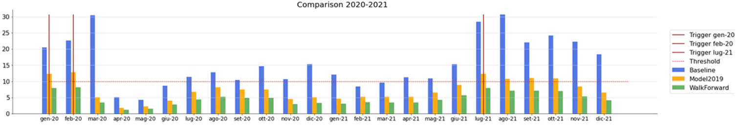
Figure 15. Baseline vs. Forecast Engine models
The effectiveness of the ‘2019 model’ and, in particular, the 2019 model with MLOps protocol is evident. The following table shows a comparison over the entire 2020-2021 period.
| Sample | Model 2019 | MlOps | Baseline | |
| Test | Media | 7.19 | 4.68 | 15.84 |
| StdDev | 3.21 | 1.95 | 7.53 | |
| Train | Media | 9.44 | 6.18 | |
| StdDev | 3.08 | 2.15 |
Conclusions
The results are definitely promising but could be further improved through the Forecast Engine with more comprehensive grid search protocols than those developed and shown in this article, using to a greater extent the hyper-parametrization functionalities made available by Keras Tuner and Optuna.
Through the Forecast Engine, further objectives can be pursued:
- replication of results on other POIs;
- verification of the possibility of obtaining adequate performance from reduced training data;
- verification of performance by moving from a formulation in terms of a supervised regression problem to a multinomial supervised classification problem. In this case the outputs (the passenger flows) will have to be discretized. The discretization strategy must necessarily depend on a defined cost function: the division into bins must generate homogeneous classes, each of which must be characterised by identical resource management in the context of an optimisation problem.
Isiway’s Forecast Engine framework is a prototype that was also developed with a view to implementation on cloud providers since:
- the engine can be replicated at script level or made available as a container;
- it is in line with the AutoML paradigm.
The protocol is based on the MLOps paradigm in a cloud environment: continuous monitoring of the model makes it possible to verify its robustness over time and, above all, automate model update procedures based on alert triggers defined from reference thresholds.