The mass use of portable devices such as smartphones and smartwatches allows us to have a complete history of our life. Thanks to the information collected by these terminals, we are able to reconstruct, with extreme accuracy, the history of our movements.
The application of machine learning algorithms to positioning data allows us to extract very relevant information useful for understanding our behavior. Some of these patterns are for example: the path we take from home to work, trips outside the city, which places we go to on Saturday nights etc ..
In this article we will describe an efficient and practical unsupervised machine learning algorithm to be able to carry out the identification of trajectory patterns. In the first part we will describe the clustering algorithm used to discover patterns, in the second one we will show how to implement this algorithm concretely in Python.
A Neuroimaging Algorithm for the Clustering of GPS Trajectories
Instead of using classic clustering algorithms like KMeans or DBSCAN, in this article we will use a cluster algorithm commonly used in brain image analysis.
QuickBundle (QB) (https://www.ncbi.nlm.nih.gov/pmc/articles/PMC3518823/pdf/fnins-06-00175.pdf) is a simple and compact clustering algorithm used to cluster matter fibers white brain extracted through the application of tractography algorithms (https://en.wikipedia.org/wiki/Tractography).
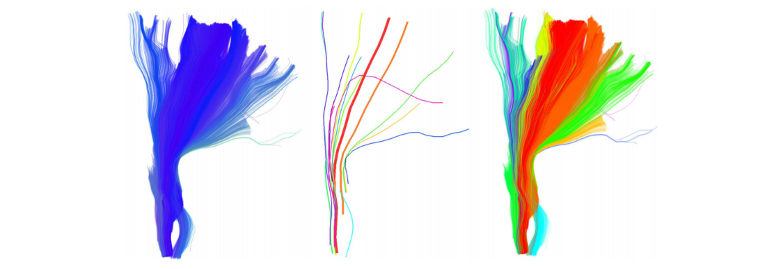
From a simple observation of the images shown below, we can easily note that GPS trajectories are very similar to white matter fibers.

Example of white matter fibers obtained by tractography algorithm.
Image from https://www.ncbi.nlm.nih.gov/pmc/articles/PMC3518823/pdf/fnins-06-00175.pdf
The main idea is to treat a single GPS trajectory as a fiber of white matter and thus unite “similar” trajectories in the same cluster. In the rest of this article we will therefore assume that Trajectory GPS = White matter fiber.
An example that shows how the algorithm is capable of grouping fibers based on their spatial trajectory, is visible in the following image.

QuickBundle centroids with different thresholds. Image from Garyfallidis et al. Frontiers In Neuroscience, vol 6, 2016.
By adjusting the threshold parameter it is in fact possible to group more or less distant fibers according to their shape. Since the behavior of the clustering algorithm is strongly dependent on the value assigned to the threshold parameter, in real application contexts it is necessary to perform a tuning of this parameter.
Another interesting result that can be derived from the algorithm is related to the ability to generate a centroid characteristic of aggregate trajectories in a given cluster. Thanks to this centroid it is in fact possible to obtain a compact representation of a group of trajectories.
Clustering of GPS Trajectories in Python
Now let’s see how to use the algorithm previously described on a real dataset of GPS trajectories using the Python language.
The data used in this article relate to the daily tracking of the movements of a given subject. The dataset, released by Microsoft Research is available at the following link (https://www.microsoft.com/en-us/download/details.aspx?id=52367). While a more detailed description is available here (https://yidatao.github.io/2016-12-23/geolife-dbscan/)
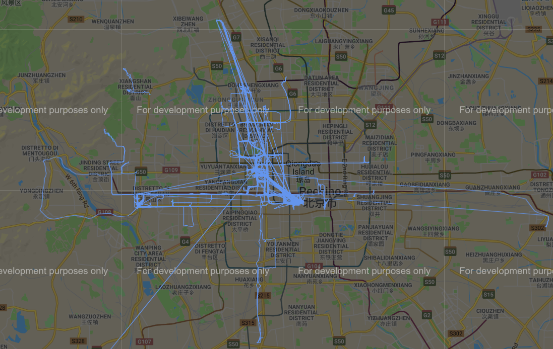
Before making a thorough analysis of the data, we carry out a plot of the GPS coordinates on google map using the gmplot library (https://github.com/vgm64/gmplot).

GPS trajectories in the dataset
So let’s start by creating a distance function that takes into account the fact that the trajectories are composed of GPS coordinates as described in the following image.

Code to calculate the distance between GPS coordinates in the trajectories
The code then calculates the distance between all pairs of points within the trajectories. It should be noted that this distance can be calculated if and only if the trajectories all have an equal number of points. Modifying this portion of code so that it is possible to calculate distance even between trajectories formed by different points is not complex.
Once we have defined how the QB algorithm must calculate the distance between the points of the trajectories, we can launch this algorithm on the reference data as described in the following image.

Python code to execute the clustering algorithm
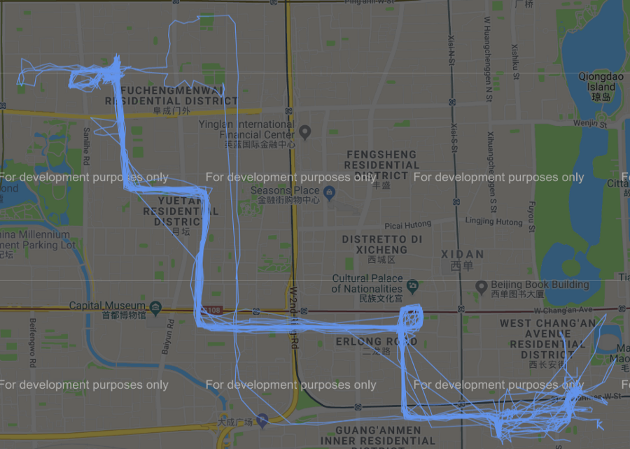
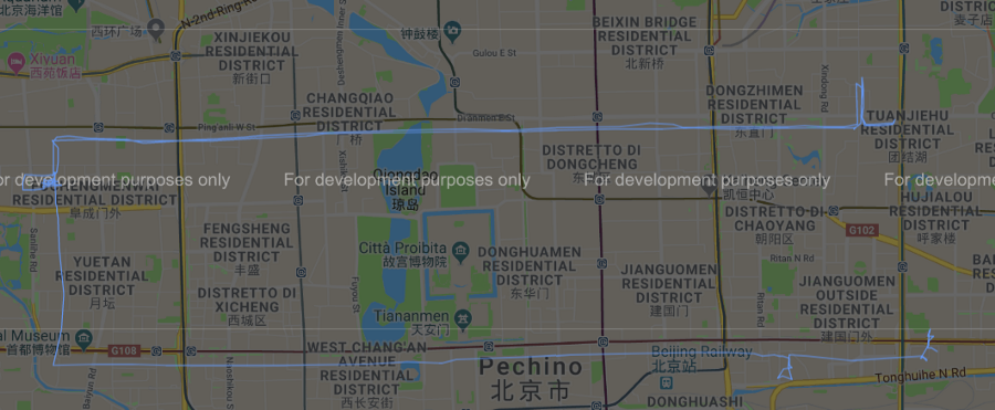
We can therefore, again with the help of gmplot, graphically represent the different clusters obtained from the application of this algorithm on google map as shown in the images below.

Cluster #0

Cluster #2

Cluster #30
Conclusion
In this article we have described a simple and fast method to cluster trajectories obtained from GPS detectors. In order to achieve this goal we used an unconventional algorithm widely used in neuroimaging.
The main limitation of this algorithm is related to the choice of the threshold parameter used. However, this problem can be easily solved through a detailed selection process.
Click for more info https://medium.com/isiway-tech/gps-trajectories-clustering-in-python-2f5874204a53

